How to calculate excited states with Qamuy
Here we take VQD (variational quantum deflation) as an example.
Install Qamuy Client SDK
If you are running this notebook on Google Colaboratory, then install Qamuy Client SDK and login to Qamuy by running the following 2 cells. Otherwise, run commands in the following 2 cells on a terminal since they require input from standard input, which cannot be handled on Jupyter Notebook.
[ ]:
!python -m pip install qamuy-client --extra-index-url https://download.qamuy.qunasys.com/simple/
Setup the input
[1]:
import qamuy.chemistry as qy
import qamuy.plot
from qamuy.client import Client

input = qy.QamuyChemistryInput()

# You can fill in your e-mail address and password.
client = Client(email_address="YOUR_EMAIL_ADDRESS", password="YOUR_PASSWORD")
Molecule
[2]:
molecule = input.target_molecule
molecule.geometry = qy.molecule_geometry(["H", "H"], [[0.0, 0.0, -0.35], [0.0, 0.0, 0.35]])
molecule.basis = "6-31g"
molecule.multiplicity = 1
molecule.sz_number = 0.0
molecule.num_excited_states = 1  # > 0 for calculating excited states
molecule.cas = qy.cas(2, 2)
[3]:
# Solver
input.solver.type = "VQD"
# or "SSVQE", "MCVQE"

# Ansatz
input.ansatz.type = "SYMMETRY_PRESERVING"
input.ansatz.depth = 4
# or "HARDWARE_EFFICIENT", "UCCSD", ...

# Optimizer
input.optimizer.type = "BFGS"
# or "SLSQP", "Adam", "NFT", "Powell", ...

# Device
input.quantum_device.type = "EXACT_SIMULATOR"
# or "SAMPLING_SIMULATOR"

# Cost Function
input.cost_function.type="SIMPLE"

# add penalties
input.cost_function.s2_number_weight=10.
input.cost_function.sz_number_weight=10.
input.cost_function.particle_number_weight=10.

# option for VQD
input.cost_function.overlap_weights = [10.]

# Post-HF methods to make a comparison
input.post_hf_methods.append(qy.PostHFMethod(type="CASCI"))
[4]:
# Chemical properties
properties = input.output_chemical_properties
properties.append(qy.output_chemical_property(target="dipole_moment", states=[0, 1]))
properties.append(qy.output_chemical_property(target="oscillator_strength", state_pairs=[[0, 1]]))
# transition_dipole_moment, gradient, hessian, non_adiabatic_coupling, ...
Run
[5]:
job = client.submit(input)
results = client.wait_and_get_job_results([job])
output = results[0].output
[Parallel(n_jobs=-1)]: Using backend ThreadingBackend with 4 concurrent workers.
[Parallel(n_jobs=-1)]: Done   1 tasks      | elapsed:   16.4s
[Parallel(n_jobs=-1)]: Done   1 out of   1 | elapsed:   16.4s finished
Get Results and Plot
[6]:
# chemical properties
q_result = output.molecule_result.quantum_device_result
print(f'S0 energy: {qy.get_evaluated_property_for_state(q_result, "energy", state=0).value}')
print(f'S1 energy: {qy.get_evaluated_property_for_state(q_result, "energy", state=1).value}')
print(f'S0 dipole moment: {qy.get_evaluated_property_for_state(q_result, "dipole_moment", state=0).value}')
print(f'S1 dipole moment: {qy.get_evaluated_property_for_state(q_result, "dipole_moment", state=1).value}')
print(f'oscillator_strength: {qy.get_evaluated_property_for_state_pair(q_result, "oscillator_strength", state_pair=(0, 1)).value}')
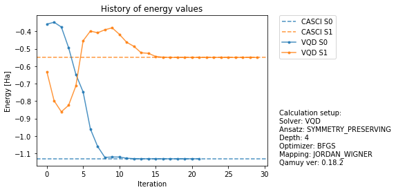
S0 energy: -1.13092554328011
S1 energy: -0.5497906158849944
S0 dipole moment: [0.0, 0.0, 9.619622851375604e-07]
S1 dipole moment: [0.0, 0.0, -8.177022843064303e-07]
oscillator_strength: 0.2067462857043951
[7]:
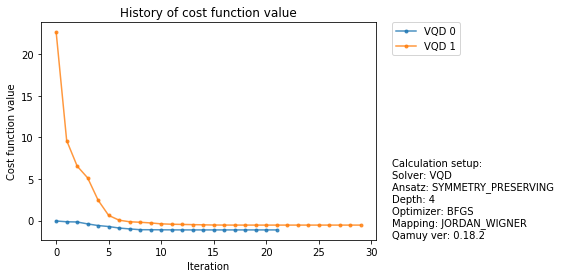
# Plot the cost function history (cost function = energy + penalty terms)
fig, ax = qamuy.plot.plot_cost_history(output)
[8]:
# Plot the energy history
fig, ax = qamuy.plot.plot_energy_history(output, state_label_map={0: "S0", 1:"S1"})