Basic usage of Qamuy SDK¶

Install Qamuy Client SDK¶

If you are running this notebook on Google Colaboratory, then install Qamuy Client SDK and login to Qamuy by running the following 2 cells. Otherwise, run commands in the following 2 cells on a terminal since they require input from standard input, which cannot be handled on Jupyter Notebook.

[ ]:

!python -m pip install qamuy-client --extra-index-url https://download.qamuy.qunasys.com/simple/

Import Qamuy¶

To use Qamuy with SDK, please import Qamuy modules.

[2]:

import qamuy.chemistry as qy
from qamuy.client import Client

# You can fill in your e-mail address and password.
client = Client(email_address="YOUR_EMAIL_ADDRESS", password="YOUR_PASSWORD")

Create Input and Run Qamuy¶

Create Input Object¶

Create a Qamuy input object.

[3]:

setting = qy.QamuyChemistryInput()

A Qamuy input object has the following structure.

QamuyChemistryInput:

target_molecule
output_chemical_properties
post_hf_methods
quantum_device
mapping
solver
ansatz
cost_function
optimizer

Set Molecule¶

Here is an example of water molecule. You can set molecular geometrical structure, basis set, active space, the number of excited state and so on.

[4]:

# H2O
atoms = ["H", "O", "H"]
coords = [
    [0.968877, 0.012358, 0.000000],
    [-0.019830, -0.025588, 0.000000],
    [-0.229801, 0.941311, 0.000000]
]

molecule = setting.target_molecule
molecule.geometry = qy.molecule_geometry(atoms, coords)
molecule.basis = "6-31g"
molecule.multiplicity = 1
molecule.num_excited_states = 0
molecule.cas = qy.cas(2, 2)

Set Chemical Properties to Be Calculated¶

You can set the chemical Properties you want to calculate here. Qamuy supports electric dipole moment, electric transition dipole moment, nuclear gradient, Hessian, vibrational frequency and nonadiabtic coupling.

[5]:

# Electric dipole moment
setting.output_chemical_properties.append(
    qy.output_chemical_property(
        target="dipole_moment", states=[0]
    )
)

Set Classical Methods for Comparison¶

Classical quantum chemistry calculation can be performed to do comparison. The available methods are MP2, CISD, CCSD, CASCI, CASSCF and FCI.

[6]:

setting.post_hf_methods.append(
    qy.PostHFMethod(type="CASCI")
)

Set Qubit Mapping¶

JORDAN_WIGNER, BRAVYI_KITAEV and SYMMETRY_CONSERVING_BRAVYI_KITAEV are available in Qamuy.

[7]:

setting.mapping.type = "JORDAN_WIGNER"

Set VQE Type¶

You can specify solver here. For computating elecronically excited state, SSVQE, MCVQE, VQD are available. You can also enable orbital optimizatin.

[8]:

setting.solver.type = "VQE"

Set Cost Function¶

The penalty term can be set to confine the number of electron, spin muliplicity and overlap in VQD.

[9]:

# Set cost function
setting.cost_function.type = "SIMPLE"
setting.cost_function.s2_number_weight = 4.0
setting.cost_function.sz_number_weight = 4.0

Set Ansatz¶

Set ansatz of electronic state. Note, you have set depth when you choose Symmetry Preserving, and trotter steps when you choose UCC and UCCSD.

[10]:

setting.ansatz.type = "SYMMETRY_PRESERVING"
setting.ansatz.depth = 4
setting.ansatz.use_random_initial_guess = True

Set Optimizer¶

Set optimizer here.

[11]:

setting.optimizer.type = "BFGS"

Set Quantum Device¶

By simply changing quantum device here, you can select state vector simulator, sampling sdimulator and real NISQ device.

[12]:

setting.quantum_device.type = "EXACT_SIMULATOR"

Run Job on Cloud¶

Submit job to Qamuy Cloud.

[13]:

job = client.submit(setting)

Get Results and Plot¶

Get Results¶

Fetch the results from Qamuy cloud.

[14]:

results = client.wait_and_get_job_results([job])
output = results[0].output

[Parallel(n_jobs=-1)]: Using backend ThreadingBackend with 8 concurrent workers.
[Parallel(n_jobs=-1)]: Done   1 tasks      | elapsed:  1.5min
[Parallel(n_jobs=-1)]: Done   1 out of   1 | elapsed:  1.5min finished

You can extract the calculated result from the ouput as follows.

[15]:

q_result = output.molecule_result.quantum_device_result
c_result = output.molecule_result.post_hf_results[0]
vqe_log = q_result.vqe_log

Ouput Structure¶

Qamuy output object has the following structure.

QamuyChemistryOutput:

input
molecule_result
- hamiltonian_generation
- hf_result
- post_hf_results
  - post_hf_log
  - evaluated_properties
- quantum_device
  - vqe_log
    - cost_hist
    - nfev
    - nit
    - opt_params
    - quantum_resources
      - circuit
      - estimated_execution_time
      - sampling
  - evaluated_properties

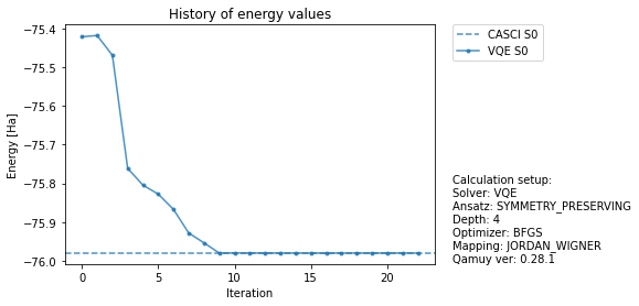
Plot Energy History¶

You can plot the energy histroy easily.

[16]:

import qamuy.plot
fig, ax = qamuy.plot.plot_energy_history(output, state_label_map={0: "S0"})

Get Chemical Properties¶

The structure of valuated_properties object is as follows.

[17]:

q_result.evaluated_properties

[17]:

[{'energy': {'values': [{'value': -75.9799236785195, 'state': 0, 'sample_std': 0.0}], 'metadata': {'elapsed_time': 0.0007705059999807418, 'success': True}}}, {'num_electrons': {'values': [{'value': 1.9999999999999996, 'state': 0}], 'metadata': {'elapsed_time': 0.0006290039999612418, 'success': True}}}, {'multiplicity': {'values': [{'value': 1.0000000000009266, 'state': 0}], 'metadata': {'elapsed_time': 0.0008784059999698002, 'success': True}}}, {'sz_number': {'values': [{'value': -1.7474910407599964e-13, 'state': 0}], 'metadata': {'elapsed_time': 0.000631903999988026, 'success': True}}}, {'dipole_moment': {'values': [{'value': [0.6539289242685531, 0.8437996784196387, 2.038928865996759e-06], 'sample_std': [0.0, 0.0, 0.0], 'state': 0}], 'metadata': {'elapsed_time': 0.0018270120000352108, 'success': True}}}]

[18]:

print("Energy:")
q_result.evaluated_properties[0].energy.values

Energy:

[18]:

[{'value': -75.9799236785195, 'state': 0, 'sample_std': 0.0}]

[19]:

print("Spin multiplicity:")
q_result.evaluated_properties[2].multiplicity.values

Spin multiplicity:

[19]:

[{'value': 1.0000000000009266, 'state': 0}]

[20]:

print("Dipole moment:")
q_result.evaluated_properties[4].dipole_moment.values

Dipole moment:

[20]:

[{'value': [0.6539289242685531, 0.8437996784196387, 2.038928865996759e-06], 'sample_std': [0.0, 0.0, 0.0], 'state': 0}]

Error Response¶

In order to look a error response, let’s make a mistake.

Setup¶

[22]:

from copy import deepcopy

setting_error = deepcopy(setting)

atoms = ["H", "Ge", "H"] #Change "O" to "Ge"
coords = [
    [0.968877, 0.012358, 0.000000],
    [-0.019830, -0.025588, 0.000000],
    [-0.229801, 0.941311, 0.000000]
]

molecule = setting_error.target_molecule
molecule.geometry = qy.molecule_geometry(atoms, coords)
molecule.basis = "6-31g"
molecule.multiplicity = 1
molecule.num_excited_states = 0
molecule.cas = qy.cas(2, 2)

Run Job¶

[24]:

#run job
job = client.submit(setting_error)

# Get results
results = client.wait_and_get_job_results([job])
output = results[0].output
error = results[0].error['error']

[Parallel(n_jobs=-1)]: Using backend ThreadingBackend with 8 concurrent workers.
[Parallel(n_jobs=-1)]: Done   1 tasks      | elapsed:   42.1s
[Parallel(n_jobs=-1)]: Done   1 out of   1 | elapsed:   42.2s finished

Show Error¶

The Error Response states “For Ge, There is no basis set of 6-31G”.

[25]:

print(error)

Traceback (most recent call last):
  File "/qamuy-cloud/.venv/lib/python3.7/site-packages/qamuy_cli/model_builder/molecular_model_builder.py", line 139, in build_molecular_model
    skip_scf=False,
  File "/qamuy-cloud/.venv/lib/python3.7/site-packages/qamuy_core/chemistry/qamuy_run_pyscf.py", line 35, in qamuy_run_pyscf
    ecp=mol_data.ecp,
  File "/qamuy-cloud/.venv/lib/python3.7/site-packages/qamuy_core/pyscf_wrappers/pyscf_wrappers.py", line 72, in compute_hf
    pyscf_mol.build(parse_arg=False)
  File "/qamuy-cloud/.venv/lib/python3.7/site-packages/pyscf/gto/mole.py", line 2346, in build
    self._basis = self.format_basis(_basis)
  File "/qamuy-cloud/.venv/lib/python3.7/site-packages/pyscf/gto/mole.py", line 2437, in format_basis
    return format_basis(basis_tab)
  File "/qamuy-cloud/.venv/lib/python3.7/site-packages/pyscf/gto/mole.py", line 422, in format_basis
    raise BasisNotFoundError('Basis not found for  %s' % symb)
pyscf.lib.exceptions.BasisNotFoundError: Basis not found for  Ge

The above exception was the direct cause of the following exception:

Traceback (most recent call last):
  File "/qamuy-cloud/.venv/lib/python3.7/site-packages/qamuy_cli/qamuycore_executor.py", line 83, in execute
    params, mo_for_hamiltonian, init_oovqe_mo
  File "/qamuy-cloud/.venv/lib/python3.7/site-packages/qamuy_cli/qamuycore_executor.py", line 185, in _build_mol_model
    init_oovqe_mo,
  File "/qamuy-cloud/.venv/lib/python3.7/site-packages/qamuy_cli/model_builder/molecular_model_builder.py", line 142, in build_molecular_model
    raise QamuyCalculationError("Molecular orbital building failed.") from e
qamuy_cli.exceptions.QamuyCalculationError: Molecular orbital building failed.

The above exception was the direct cause of the following exception:

Traceback (most recent call last):
  File "/qamuy-cloud/.venv/lib/python3.7/site-packages/qamuy_cli/__main__.py", line 125, in main
    s3_folder,
  File "/qamuy-cloud/.venv/lib/python3.7/site-packages/qamuy_cli/utils/run.py", line 34, in run_all
    s3_folder,
  File "/qamuy-cloud/.venv/lib/python3.7/site-packages/qamuy_cli/utils/run.py", line 65, in run_compute
    s3_folder=s3_folder,
  File "/qamuy-cloud/.venv/lib/python3.7/site-packages/qamuy_cli/qamuycore_executor.py", line 86, in execute
    raise QamuyCalculationError("Build molecular model failed") from e
qamuy_cli.exceptions.QamuyCalculationError: Build molecular model failed

Sampling Simulator¶

Prepare Input¶

For changing to sampling simulator is easy, just change quantum device.

[26]:

setting_sampling = deepcopy(setting)
setting_sampling.quantum_device.type = "SAMPLING_SIMULATOR"
setting_sampling.observable_grouping.type = "BITWISE_COMMUTING"
setting_sampling.sampling_strategy.type = "WEIGHTED"
setting_sampling.sampling_strategy.num_total_shots = 1e6
setting_sampling.sampling_strategy.shot_unit = 1

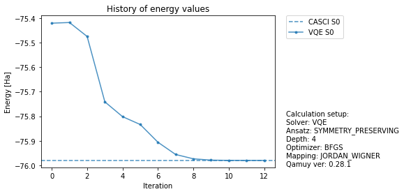
Run Job and Plot¶

Run job and plot are same with the case of state vector simulator.

[33]:

# run job
job = client.submit(setting_sampling)

# Get results
results = client.wait_and_get_job_results([job])
output = results[0].output

# Extract results
q_result = output.molecule_result.quantum_device_result
c_result = output.molecule_result.post_hf_results[0]
vqe_log = q_result.vqe_log

[Parallel(n_jobs=-1)]: Using backend ThreadingBackend with 8 concurrent workers.
[Parallel(n_jobs=-1)]: Done   1 tasks      | elapsed:   37.0s
[Parallel(n_jobs=-1)]: Done   1 out of   1 | elapsed:   37.0s finished

[34]:

import qamuy.plot
fig, ax = qamuy.plot.plot_energy_history(output, state_label_map={0: "S0"})

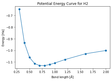
Potential Energy Curve¶

Setup¶

[29]:

distance_list = [0.3, 0.4, 0.5, 0.6, 0.7, 0.8, 0.9, 1.0, 1.2, 1.6, 2.]

jobs = []
for distance in distance_list:
    new_input = deepcopy(setting)
    new_input.target_molecule.geometry = qy.molecule_geometry(["H", "H"], [[0.0, 0.0, - distance / 2], [0.0, 0.0, distance / 2]])
    jobs.append(client.submit(new_input))

[30]:

results = client.wait_and_get_job_results(jobs)
outputs = [res.output for res in results]

[Parallel(n_jobs=-1)]: Using backend ThreadingBackend with 8 concurrent workers.
[Parallel(n_jobs=-1)]: Done   2 out of  11 | elapsed:   21.3s remaining:  1.6min
[Parallel(n_jobs=-1)]: Done   4 out of  11 | elapsed:   31.7s remaining:   55.5s
[Parallel(n_jobs=-1)]: Done   6 out of  11 | elapsed:   36.9s remaining:   30.8s
[Parallel(n_jobs=-1)]: Done   8 out of  11 | elapsed:   36.9s remaining:   13.9s
[Parallel(n_jobs=-1)]: Done  11 out of  11 | elapsed:   47.8s finished

[31]:

energy_list=[output.molecule_result.quantum_device_result.evaluated_properties[0].energy.values[0].value for output in outputs]

[32]:

import matplotlib.pyplot as plt

plt.plot(distance_list,energy_list, "o-")
plt.xlabel("Bond length [$\AA$]")
plt.ylabel("Energy [Ha]")
plt.title("Potential Energy Curve for H2")
plt.show()